CS 4641 Final Project Team 35: Mushroom Classification
Background and Problem Definition
Mushrooms are a staple food in many parts of the world. However, we have always been cautioned to never eat wild mushrooms since many mushrooms can be poisonous and induce serious symptoms such as seizures, hallucinations, breathing difficulties, kidney/liver failure, coma, or death. In fact, according to The National Poison Data System (NPDS) from 1999 to 2016, 133700 cases, or roughly 7428 cases per year, of mushroom exposure have been reported [1]. This staggering statistic coupled with a recent trend of mushroom hunting (or “shrooming”) makes it even more imperative that we can accurately identify which mushrooms are edible and which ones are inedible.
A way we can classify if a mushroom is edible or not is by looking at the physical features of the mushroom itself. However, with such a wide variety of mushrooms available, the classification is not as simple as looking at a single feature to determine how edible the mushroom is. Instead, we would have to consider many if not all of the features of the mushroom to make a definite conclusion.
Therefore, for this project, our objective is to create a machine learning model that can predict how edible a mushroom is based on the physical features of the mushrooms as accurately as possible. This will not only be a useful and convenient tool for mushroom hunters, but can also prevent people from mistakenly ingesting a potentially toxic mushroom.
Overview of the Dataset
To approach this problem, we decided to use a public domain dataset that was provided by The Audubon Society Field Guide to North American Mushrooms. This dataset consists of descriptions of hypothetical samples corresponding to 23 species of gilled mushrooms. Although this dataset is nearly 30 years old, it is still relevant since the question of classifying mushrooms based on their edibility remains unanswered. This dataset has 8124 entries and each entry has 23 attributes. The class attribute corresponds to the edibleness of the mushroom (either edible or poisonous). The remaining 22 attributes are used to specify the physical appearance of each mushroom. These attributes are: cap-shape, cap-surface, cap-color, bruises, odor, gill-attachment, gill-spacing, gill-size, gill-color, stalk-shape, stalk-root, stalk-surface-above-ring, stalk-surface-below-ring, stalk-color-above-ring, stalk-color-below-ring, veil-type, veil-color, ring-number, ring-type, spore-print-color, population, and habitat. Figure 2.1 shows the statistics of these features:
| count | # of unique labels | Most common label | Frequency of most common label | |
| class | 8124 | 2 | e | 4208 |
| cap-shape | 8124 | 6 | x | 3656 |
| cap-surface | 8124 | 4 | y | 3244 |
| cap-color | 8124 | 10 | n | 2284 |
| bruises | 8124 | 2 | f | 4748 |
| odor | 8124 | 9 | n | 3528 |
| gill-attachment | 8124 | 2 | f | 7914 |
| gill-spacing | 8124 | 2 | c | 6812 |
| gill-size | 8124 | 2 | b | 5612 |
| gill-color | 8124 | 12 | b | 1728 |
| stalk-shape | 8124 | 2 | t | 4608 |
| stalk-root | 8124 | 5 | b | 3776 |
| stalk-surface-above-ring | 8124 | 4 | s | 5176 |
| stalk-surface-below-ring | 8124 | 4 | s | 4936 |
| stalk-color-above-ring | 8124 | 9 | w | 4464 |
| stalk-color-below-ring | 8124 | 9 | w | 4384 |
| veil-type | 8124 | 1 | p | 8124 |
| veil-color | 8124 | 4 | w | 7924 |
| ring-number | 8124 | 3 | o | 7488 |
| ring-type | 8124 | 5 | p | 3968 |
| spore-print-color | 8124 | 9 | w | 2388 |
| population | 8124 | 6 | v | 4040 |
| habitat | 8124 | 7 | d | 3148 |
Figure 2.1 shows some statistics about the features in the dataset.
We note that veil-type has only 1 unique label and therefore can be disregarded entirely from the dataset. We also note that the gill-color feature has a relatively small frequency for its most frequent label indicating the feature may be important.
Based on Figure 2.1, we determine that it is possible for each feature to have multiple (>2) labels since attributes such as gill-color and ring-type can have many unique labels.
To assess the viability of the dataset, we look at how many edible and poisonous mushrooms are provided. If the number of edible and poisonous mushrooms are roughly the same, we know we have a good representation of edible and poisonous mushrooms to train our models. Figure 2.2 below shows that the dataset is viable and balanced
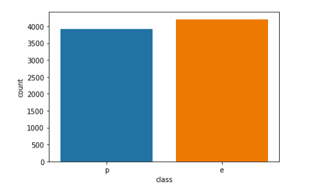
Figure 2.2 indicates that the dataset contains 4208 edible mushrooms and 3916 poisonous mushrooms
We also investigated further and saw there were no null values for any of the entries. This can be seen in Figure 2.1 since the count of all the labels in each feature is equal to the total number of entries in the database. This makes it easier to run models on as all entries are 100% valid and accurately filled in and we do not have to perform additional data-preprocessing. The number of unique features for each dataset is also something we could look at since it is one of the factors in determining entropy. Figure 2.3 shows the number of unique labels each feature in the dataset has:
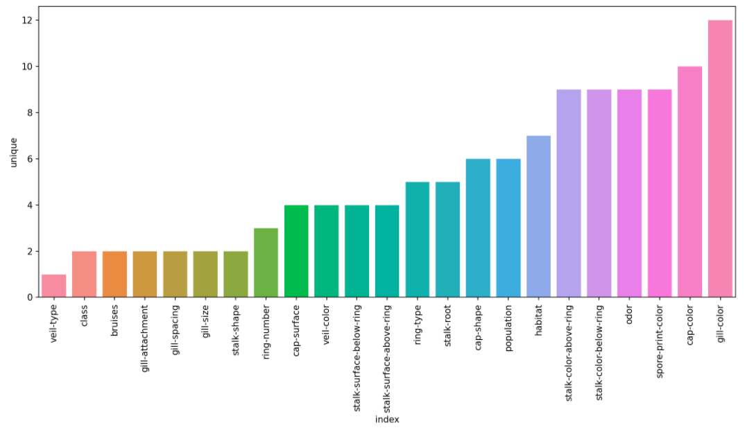
Figure 2.3 shows the unique labels each feature has
The features on the right should play a good role in the classification.
Methodology
To begin with the classification process, we first performed dataset preprocessing:
1. Data Preprocessing
We have determined that our dataset is in fact balanced and usable. However, one issue that we can immediately see is that the dataset does not contain any numerical data. All the data is categorical and running machine models using categorical data is often very difficult if not impossible. To remedy this issue, we employed two ways to convert our dataset into one with numerical features: dummy coding and the OrdinalEncoder in Python’s sklearn library. We expect different results on these generated datasets when we perform data-preprocessing.
OrdinalEncoder
| class | cap-shape | cap-surface | cap-color | bruises | odor | gill-attachment | ... | |
| 0 | 1.0 | 5.0 | 2.0 | 4.0 | 1.0 | 6.0 | 1.0 | ... |
| 1 | 0.0 | 5.0 | 2.0 | 9.0 | 1.0 | 0.0 | 1.0 | ... |
| 2 | 0.0 | 0.0 | 2.0 | 8.0 | 1.0 | 3.0 | 1.0 | ... |
| 3 | 1.0 | 5.0 | 3.0 | 8.0 | 1.0 | 6.0 | 1.0 | ... |
| 4 | 0.0 | 5.0 | 2.0 | 3.0 | 0.0 | 5.0 | 1.0 | ... |
Dummy Variable
| cap-shape_b | cap-shape_c | cap-shape_f | cap-shape_k | cap-shape_s | cap-shape_x | cap-surface_f | ... | |
| 0 | 0 | 0 | 0 | 0 | 0 | 1 | ... | |
| 1 | 0 | 0 | 0 | 0 | 0 | 1 | ... | |
| 2 | 1 | 0 | 0 | 0 | 0 | 0 | ... | |
| 3 | 0 | 0 | 0 | 0 | 0 | 1 | ... | |
| 4 | 0 | 0 | 0 | 0 | 0 | 1 | ... |
Figure 3.1 shows the results of the data conversion. The top table is the results of applying OrdinalEncoder and the bottom table is the results of applying the dummy variable method (Note: features have been omitted from both tables due to space and we only show the first 5 entries of the database)
To perform data preprocessing, there are 2 dimensionality reduction techniques we can use, PCA (Principal component analysis) and MCA (Multiple Correspondence Analysis). Generally PCA algorithms are applied on continuous datasets.
First, we apply PCA for 2 variables on both of the converted datasets to determine which data conversion method is ideal for this dataset. When PCA is applied, the percentage variance in the dummy data method for the selected feature 1 and feature 2 is 0.08891017 and 0.08125474, respectively. However, the percentage variance in the OrdinalEncoder method for the selected feature 1 and feature 2 is 0.19017657 and 0.1257281, respectively. The total variance captured by either of the datasets is not very high for 2 variables. However, the total variance is definitely much higher for the OrdinalEncoder data as compared to the dummy variable data. The clustering possibility is also not very satisfactory though each algorithm does give us some clusters that are unique to a class as shown in Figure 3.2:
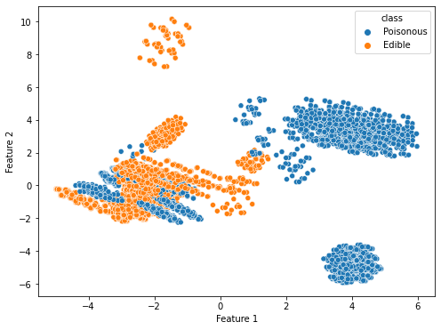
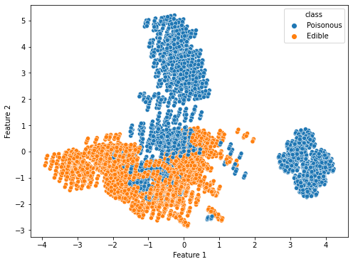
Figure 3.2 shows the PCA results on the converted datasets. The left figure is the results of the dummy data method and the right figure is the results of using the OrdinalEncoder method
Because the variances for both methods are so low for 2 variables, we want to know how many variables we need to have to have at a minimum total variance of 0.95. We calculate that the number of features we require to meet our requirements for the OrdinalEncoder dataset is 16. The number of features we require to meet our requirements for the dummy variable dataset is 59. We graph the variance distribution based on the number of features selected for each of the databases to determine performance as shown in Figure 3.3 below.
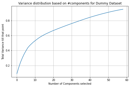
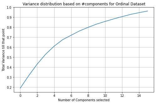
Figure 3.3 shows the variance distribution based on the number of features selected for the dummy dataset (top) and OrdinalEncoder dataset (bottom)
Based on the graph, we see that the OrdinalEncoder dataset’s slope curves slower than the dummy variable dataset. The OrdinalEncoder dataset has a much better performance in terms of variance maximization with the least number of features.
Another data preprocessing technique we can use is Multiple Correspondence Analysis (MCA). MCA is generally used for nominal categorical data, which fits our dataset more closely. However, when MCA is applied, the variances, or inertia, as it is called in MCA, for the selected feature 1 and feature 2 is 0.0807 and 0.0725, respectively, which is still low. Plotting the MCA data, we get the following visualization:
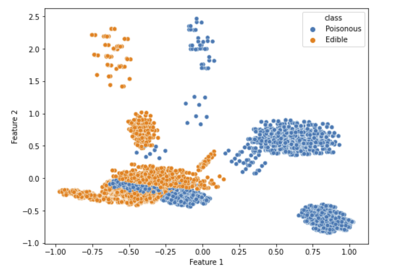 Figure 3.4 shows the MCA results and distribution on the converted dataset.
From the plot, despite MCA being intended for nominal categorical data, it is clear that the distribution is not very good. One potential cause for this is that MCA is using one hot encoded version of a dataset on CA. Let’s plot inertia relative to the number of components and compare the results to PCA.
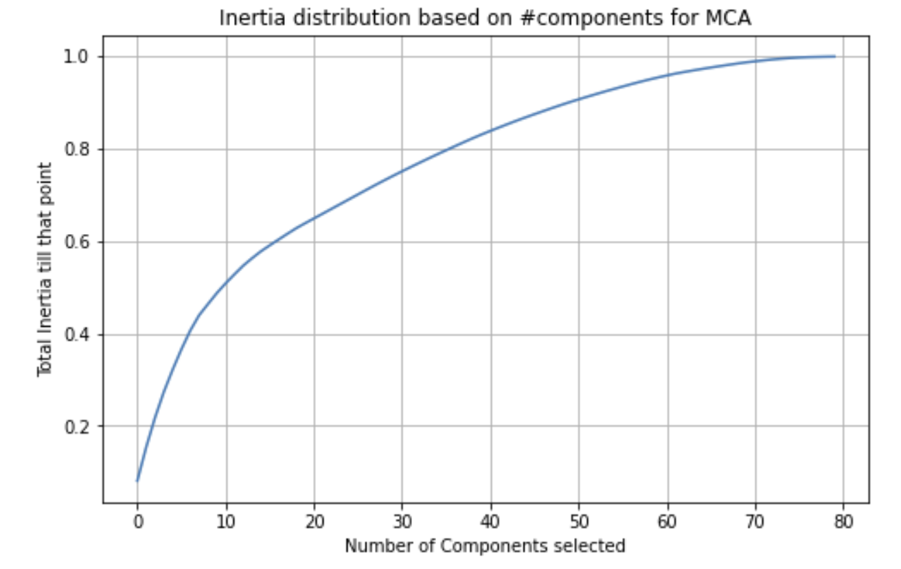 Figure 3.5 shows how variance increases relative to the number of components selected for MCA
The number of components required to reach an inertia (variance) of 0.95 is 59. Clearly, running PCA on the OrdinalEncoder has a much higher performance relative to MCA. Another thing to note about Figure 3.5 is that the graph converges to 1 much quicker than some of the other dimensionality reduction techniques we have seen.
2. ML Model Results & Discussion
Now that we have applied preprocessing techniques to our data, we can run some models on it. The first model we will use on our data is Naive Bayes, which uses the distribution P(X_i,y)/P(y) in the Bayes rule calculation. We will run Naive Bayes with several different distributions, and also use our preprocessed data, and compare the results.
First, we run a Gaussian Naive Bayes, classifying each of the test data as either poisonous or edible.
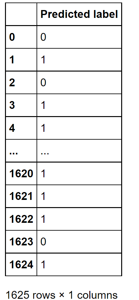
Figure 4.1 shows the classification of each test data after Gaussian Naive Bayes is run, with each data point being labeled as either poisonous or edible.
Doing so yields a surprisingly high accuracy of 91.57%. The results can be visualized through a confusion matrix.
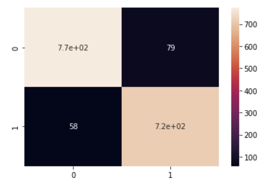
Figure 4.2 shows the confusion matrix of running a Gaussian Naive Bayes on the data
From Figure 4.2 the true positives and true negatives are much greater in magnitude than the false positives and negatives, which matches our high accuracy of about 92%.
Next, we see if we can do better by running the same Gaussian Naive Bayes model, except on the data preprocessed with MCA. Unfortunately, doing so yields an accuracy of about 19%, which is quite worse than before. This follows from the worse distribution that MCA gave us as explained earlier. The results can be visualized through the following confusion matrix.
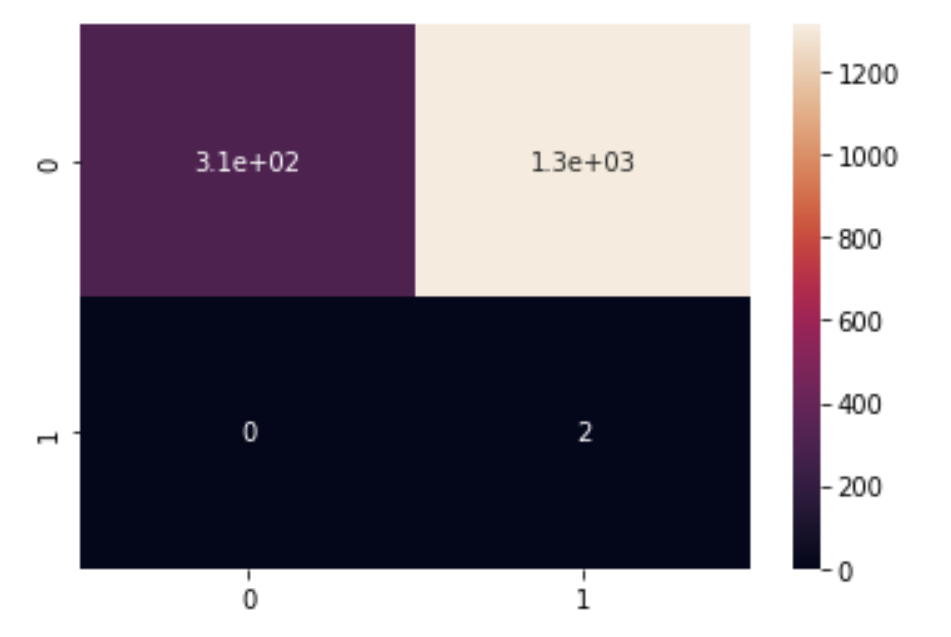
Figure 4.3 shows the confusion matrix of running a Gaussian Naive Bayes on the data after it is preprocessed using MCA
From Figure 4.3, we see that the number of false positives has skyrocketed, while the number of false negatives has dropped to zero. Clearly, this strategy didn’t work out, so we take a different approach.
Our data is being grouped into two sets, either poisonous or edible, so perhaps Categorical Naive Bayes, which assumes a Categorical Distribution, would be a better candidate for the data. Fortunately, our intuition was correct, with Categorical Naive Bayes yielding an accuracy score of 96.5%, an increase of almost 5% from Gaussian Naive Bayes! The results can be analyzed more thoroughly through the confusion matrix.
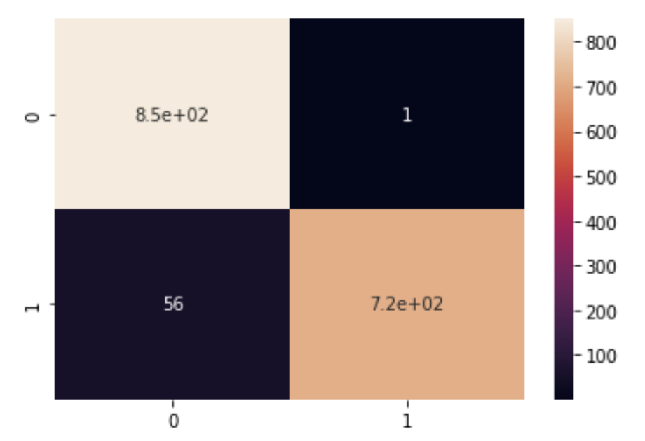
Figure 4.4 shows the confusion matrix for the Categorical Naive Bayes Model
Relative to Gaussian Naive Bayes, the areas that were improved upon in Categorical Naive Bayes were increasing the True positive rate while decreasing the False Positive rate.
Though it is apparent that Categorical Naive Bayes represents our data very well, let’s examine how other distributions impact Naive Bayes accuracy, as the choice of distribution seems to have a large impact on the performance.
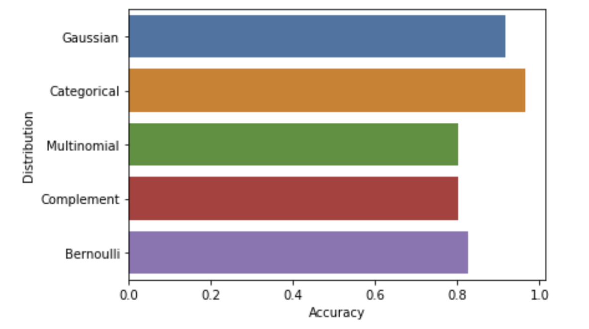
Figure 4.5 shows the accuracy of a Naive Bayes model on the data using assuming different types of distributions
From Figure 4.5, we can see that a Categorical distribution yields the highest accuracy, which matches our specific dataset, as the data is grouped into two sets.
Though categorical distribution is very effective, we can still apply other classification models on the dataset. We can implement a decision tree which works by continuously splitting the data using specific conditions. We first implement a simple decision tree on our data and calculate the confusion matrix, both of which can be seen in Figure 4.6:
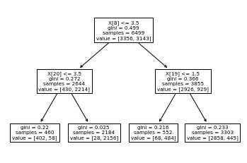
Figure 4.6 shows the implementation of a basic decision tree on the dataset and its confusion matrix
Based on the results of the decision tree, there is an overwhelmingly large number of true positives and true negatives, with very few false positives. The accuracy for this unoptimized decision tree was 92.31%. Therefore, it seems like our data set appears to be particularly well suited for supervised machine learning models. In this example, we set the max tree depth to be quite small. Though the small max tree depth makes overfitting unlikely, we can still optimize maximum depth and increase accuracy. We optimized the maximum depth parameter and determined a value of 7. The confusion matrix result is shown in Figure 4.7.
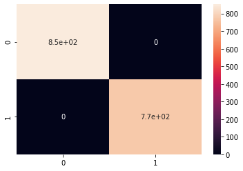
Figure 4.7 shows the confusion matrix results of the decision tree with a maximum depth of 7 on the dataset. Note the 100% accuracy
Shockingly, we received no false positives or false negatives resulting in a 100% accuracy. This is significant as we do not want to classify a poisonous mushroom as edible even by mistake.
Therefore using 20% of our data for training purposes and 80% of our data for testing purposes, our optimized decision tree perfectly captures the data. In other words, all mushrooms that should be predicted edible are accurately predicted to be edible, and all mushrooms that are poisonous are accurately predicted to be poisonous. Though we have achieved a very successful 100% accuracy, we should always treat such results with skepticism and caution. To study our dataset more, we used different testing and training data splits. We predict it is unlikely that such a high accuracy is maintained as the model is trained with a lesser percentage data. A diagram showing these results is displayed in Figure 4.8:
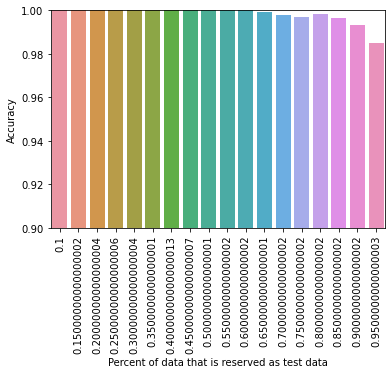
Figure 4.8 displays the accuracy results in using our optimized decision tree model with differing levels of testing and training data splits.
These results are impressive and show that the optimized decision tree classification method can perform pretty well (98.5% accuracy) with only 5% training data and 95% testing data. We also considered implementing an ensemble of decision trees, or a random forest classification method, even though it is unnecessary at this point. We were interested in the benefits of using a random forest since decision trees often perform very well when they are part of a random forest. Using a simple, unoptimized model we achieved 100% accuracy using 20% of our data for training purposes and 80% of our data for testing purposes. Figure 4.9 below displays the results of using different testing and training data splits:
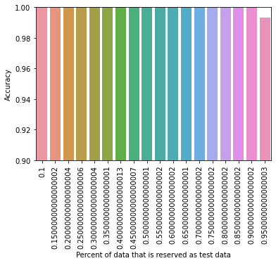
Figure 4.9 displays the accuracy results in using a non-optimized random forest classification model with differing levels of testing and training data splits.
These results are even more astonishing than the optimized decision tree model’s results. Our accuracy remains at 100% despite only having 10% training data and 90% testing data. Using only 5% of our data as training data and 95% of our data as testing data, we achieve an accuracy of 99.33%.
We also decided to optimize this model for the best results. After optimizing the n_estimators parameter to be 1601, and the max_depth parameter of each tree to be 76, we charted the accuracy against different test/train splits. This time, our improvement was not very drastic and we achieved a minute increase in accuracy to 99.57%.
Finally, to test our knowledge of neural networks, we implemented a neural network to perform classification on this dataset and compared to how it performs in comparison with the baseline and some of these mother models that we have implemented already. To start, we found that the method most suited towards a classification task is compiling our neural network by using the Adam Optimizer Algorithm and a binary cross entropy loss function. Note that we used 4 layers in our neural network. With 10 epochs, a batch size of 100 and using 20% of our data for training purposes and 80% of our data for testing purposes, we immediately achieved 100% accuracy. This indicates that a neural network also performs exceptionally well to perform classification tasks on this dataset.
Having achieved 100% accuracy with the models implemented, it seems redundant and unnecessary to implement any other further complex models on our dataset.
Conclusions
Figure 5.1 below is a summary of the models we implemented and ran against our dataset using 20% of our data for training purposes and 80% of our data for testing purposes:
| Classification Method | Accuracy (%) |
| Gaussian Naive Bayes (with PCA preprocessing) | 91.57 |
| Categorical Naive Bayes | 96.5 |
| Unoptimized Decision Tree | 92.31 |
| Optimized Decision Tree | 100 |
| Unoptimized Random Forest | 100 |
| Optimized Random Forest | 100 |
| Neural Network | 100 |
Figure 5.1 shows a summary of the accuracies received from the 8 classification models we studied with 20% of our data for training purposes and 80% of our data for testing purposes.
We noticed that we achieved excellent initial success using simple models like Naive Bayes and decision trees. Therefore, we believe that this dataset has key attributes that make prediction easy. Looking at our data-preprocessing may help with determining if this is true. In our pre-processing using PCA and MCA (Figure 3.3 and 3.4), the visuals show that the poisonous and edible mushrooms are not scattered randomly, but are instead clumped together rather tightly. This means that in our dataset, if there is a poisonous mushroom, it is extremely likely that there is another poisonous mushroom that shares very similar characteristics. Likewise, if there is an edible mushroom, it is extremely likely that there is another edible mushroom that shares very similar characteristics. The absence of outliers from the PCA and MCA visuals are a proof of this fact. This can explain why the results for our models have such high accuracy and a low amount of false positives and false negatives.
If we compare our results to some other models out there implemented on this dataset, we see that the results match. Many other models do indeed have close to 100% accuracy on the dataset. The unique perspective we bring to the table is the addition of analysis with a training dataset that is of a lower percentage. We have compared the results when the training dataset is only 5% of the data and when it is 20% of the data, and found that the reduction in accuracy is not huge. This leads us to the conclusion that, for this dataset, a low percentage of data is a good representation of the entire dataset. There is not much variation in the entire dataset, and that is why choosing a lower number of data points also does not lead to a great reduction in accuracy. This regularity and predictablity in the dataset could be one of the reasons for why we are getting such high accuracy for the models we have applied.
To reconfirm our beliefs, we tested multiple more complex models and arrived at results that supported our predictions. Since this high level of accuracy can be achieved by using simpler models, it is likely that real-world applications would favor such simpler models instead of implementing complex and expensive machine learning models. In other words, even though we have achieved better performance with a random forest and a neural network than a decision tree, it is likely that in practice we would opt for a simpler model such as the optimized decision tree. This is because in comparison to the more complex models the reduction in accuracy is very minute and almost unnoticeable and the complexity, computing power, and time required to run the more advanced models is high. The accuracy for the decision tree using 20% of our data for training purposes and 80% of our data for testing purposes is at 100% which is undeniably extremely good. All in all, we were successful in creating a machine learning model that yielded very high accuracy on this dataset and are hopeful that this model is applicable to those studying the ediblity of mushrooms.